Lunchtime Hack: Decoding LocationHistory
Last month we took a look at how we might get our location history from Google and show it on a map. We found that the real deal is found at Takeout and consists of a file that's mostly an array of lat/lng/time entries, but with some sort of 'activities' sub-elements sometimes. After a quick glance I just munged it all together and went on, but recently I had another look to check assumptions (radical!). Here's what I found:
- Sometimes there is also an accuracy, velocity, heading and altitude.
- The 'activitys' element is a bit of a mystery.
- About 1/3 of entries have one or more of them.
2. Each consisting of a timestamp and then a bunch of \'activities\', where activities are like
    `{"type" : “still”, "confidence" : 100}`

    which looks similar to
    [DetectedActivity](https://developer.android.com/reference/com/google/android/gms/location/DetectedActivity.html)
    from Android
There are lots of timestamps
$ grep timestampMs LocationHistory.json | wc -l
   1045241
But many are repeats
$ grep timestampMs LocationHistory.json | sort | uniq -d | wc -l
   611
I investigated a few of these, and they were something like
    "timestampMs" : "1408910152294","latitudeE7" : xx599,"longitudeE7" : xx279,"accuracy" : 26,
      "activitys" : [ {"timestampMs" : "1408910091630", "activities" : [ yyy ]} ]
    }, {
      "timestampMs" : "1408910091344","latitudeE7" : xx599,"longitudeE7" : xx279,"accuracy" : 26,
      "activitys" : [ {"timestampMs" : "1408910091630", "activities" : [ yyy ]} ]
So the 'activity' is at the same time, at the same lat/lng location, but the top-level groups have different timestamps (in this case about a minute apart). I've no idea whey.
Now, let's start playing with some new hammers I've found to see what we can find that looks like a nail. jq is my first hammer of the day.
There are repeated lat/log pairs
$ jq '.locations[] | [.latitudeE7 , .longitudeE7] | tostring' < LocationHistory.json |  wc -l
   691189
But again, a number of them are repeated
$ jq '.locations[] | [.latitudeE7 , .longitudeE7] | tostring' < LocationHistory.json | sort | uniq -d | wc -l
   57649
So we don't have a particular index. It seems to be just collections of detected activities at a location, at around the same time. And there may be more than one of these clusters for any given location
Time for another hammer! Pandas apparently has a good datatable that we might be able to use. A quick look shows a 1000 page manual, so I actually spent a few train commutes reading. But!
$ ipython --pylab
  <stuff>
  In [1]: from datetime import datetime, timedelta
  In [2]: import math, json, pandas.tools.plotting, urllib2
First, grab the file
In [3]: j = json.load(urllib2.urlopen("https://dl.dropboxusercontent.com/u/xxxxx/LocationHistory.json"))['locations']
Then stick it in an array, with some light conversions. But pull out those activities and add them to the array in their own right. Keep track of numbers of activities and 'activitys' to see what we find. Also track that diff between the group timestamp and activity timestamp.
In [4]: d = []
In [5]: for i in j:
    ...:         r = i.copy() # leave j alone. We will want to re-analyse without having to reload.
    ...:         a = i.get('activitys', [])
    ...:         r['timestampMs'] = int(r['timestampMs'])
    ...:         r['len_activitys'] = len(a)
    ...:         r['longitudeE7'] = float(r['longitudeE7']) / 10**7
    ...:         r['latitudeE7'] = float(r['latitudeE7']) / 10**7
    ...:         r['activities'] = ''
    ...:         r['timestampDiff'] = 0
    ...:         d.append(r)
    ...:         for k in a:
    ...:                     nr = r.copy()
    ...:                     nr['len_activities'] = len(k['activities'])
    ...:                     nr['len_activitys'] = 0
    ...:                     nr['timestampDiff'] = (r['timestampMs'] - int(k['timestampMs']))
    ...:                     nr['activities'] = ','.join([v['type']+':'+str(v['confidence']) for v in k['activities']])
    ...:                     d.append(nr)
    ...:
Into the dataframe
In [6]: import pandas as pd
In [7]: df = pd.DataFrame(d)
In [8]: df['timestampDiff'] = df['timestampDiff'] / 3600000.0 # make it hours
In [9]: df.describe()
Out[9]:
              accuracy      altitude       heading      latitudeE7  \
count  1045169.000000  27544.000000  20947.000000  1045241.000000
mean        86.618834     66.001997    167.908961       44.210958
std        309.453940    108.628497     98.520943       23.518421
min          0.000000   -433.000000     -1.000000      -35.824186
25%         20.000000     46.000000     92.000000       51.375634
50%         25.000000     64.000000    148.000000       51.375675
75%         37.000000     78.000000    252.000000       51.502468
max      85584.000000   5164.000000    359.000000       60.442490

        len_activities   len_activitys     longitudeE7   timestampDiff  \
count   354052.000000  1045241.000000  1045241.000000  1045241.000000
mean         1.459554        0.338728       12.997212        0.557364
std          1.020959        1.479987       41.965071      418.273763
min          1.000000        0.000000     -115.175744       -7.957426
25%          1.000000        0.000000       -0.436147        0.000000
50%          1.000000        0.000000       -0.436057        0.000000
75%          1.000000        1.000000       -0.081249        0.000000
max          7.000000      446.000000      151.286411   381569.052487

        timestampMs      velocity
count  1.045241e+06  25323.000000
mean   1.378485e+12      5.184931
std    2.343113e+10      6.857069
min    1.258022e+12     -1.000000
25%    1.366824e+12      0.000000
50%    1.382006e+12      1.000000
75%    1.394385e+12      8.000000
max    1.409141e+12     47.000000
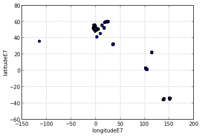
Ok. So we see that the timestampDiff is mostly quite small, with huge outliers. But let's start by plotting all the positions in a scatter plot. Here's where I've been -- minimalist style!
In [10]: df.plot('longitudeE7','latitudeE7',kind='scatter', figsize=(6, 4))
Out[10]:
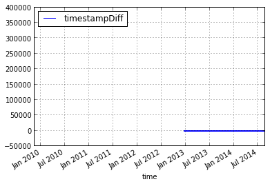
I'm still interested in those timestamp differences. Let's plot them, against the actual timestamp.
In [11]: df['time'] = pd.to_datetime(df['timestampMs'], unit='ms')
In [12]: pldf = df[['timestampDiff', 'time' ]]
In [13]: pldfi = pldf.set_index('time')
In [14]: pldfi.plot()
Out[14]:
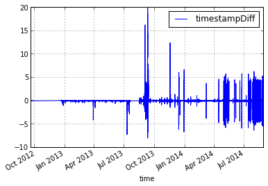
Outliers. Cut them off and try again.
In [15]: pldfi = pldfi[pldfi.timestampDiff < 150000]
In [16]: pldfi.plot()
Out[16]:
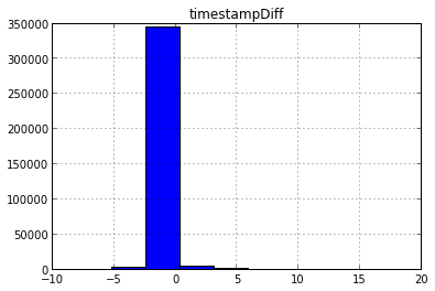
A little more informative, but only in as much as I can't see a pattern so I'll probably ignore them. Let's check with a histogram.
In [17]: pldfi.hist()
Out[17]: array([[Axes(0.125,0.125;0.775x0.775)]], dtype=object)
Ok. So mostly small. Well, let's cut the dataset down to a box bounded by slightly outside the two ends of my cycle route. And then save all activities that are onBicycle to a some sort of json thing.
In [18]: lshiftLoc = {'tl':(51.527530, -0.082466), 'br':(51.526702, -0.079849)}
In [19]: wlooLoc = {'tl':(51.504162, -0.114610), 'br':(51.499781, -0.110748)}
In [20]: dfCut = df[(df.latitudeE7 < lshiftLoc['tl'][0])
    ....:           (df.latitudeE7 > wlooLoc['br'][0])
    ....:           (df.longitudeE7 < lshiftLoc['br'][1])
    ....:           (df.longitudeE7 > wlooLoc['tl'][1])]
In [21]: dfBicycle = df[df['activities'].str.contains('onBicycle')]
In [22]: dfBicycle = dfBicycle[['timestampMs', 'latitudeE7', 'longitudeE7']]
In [23]: dfBicycle.index = dfBicycle['timestampMs']
In [24]: dfBicycle = dfBicycle[['latitudeE7', 'longitudeE7']]
In [25]: dfBicycle = dfBicycle.iloc[len(dfBicycle)::-1]
In [26]: dfBicycle.to_json('bicycles.json')
Which then fails because the index (timestampMs) is not unique. Ok. Time to stop and eat.
So, what have I accomplished? I learned a bit about some tools. I learned almost nothing about the LocationHistory format.
<rant>
I think that google takeout is an awesome thing. That sort of openness and non-stickyness from a large company is unusual, and to be applauded. And mostly they seem to be sticking with well known file formats that are documented and can be re-used in other services, but not with location history. I'm guessing it's just a combination of a lack of common file formats to choose from coupled with a developer's love of writing documentation, rather than whatever motivated Microsoft to produce .docx. But if someone on the inside could throw us a note about what it's all about, that'd be really nice.
</rant>
(Originally here)


